Grapes
Crop Coefficient
Comparison of Methods for Computing a Crop Coefficient for Grapes
See Evans et al. 1993 for cutoff temperatures for grapes and Crop coefficient based on growing degree days
The crop coefficient (Kc) is a parameter used by various irrigation scheduling methods to scale potential evaporation and transpiration (evapotranspiration) to the actual levels for the particular crop. The crop coefficient (Kc) is usually computed as a function of total accumulated growing degree days. The value of Kc for grapes was obtained by fitting a function to theoretical data obtained from:
* Crop Water Requirements
  FAO Irrigation and Drainage Paper 24

  Pg 50, Table 27: Kc Values for Grapes (Clean Cultivated,
  Infrequent Irrigation, Soil Surface Dry Most of the Time)

  Using the data for areas of only light frosts, ground cover of 30-35 percent,
  with dry and light to moderate wind conditions.
The Growing Degree Days data was computed using 1995 Data in Las Cruces, NM, using both the averaging and the single sine methods of computation. The Growing Degree Days were calculated using the following parameters:
*
  Upper Threshold:  30°C
  Lower Threshold:  10°C
  Lower Cutoff:     10°C
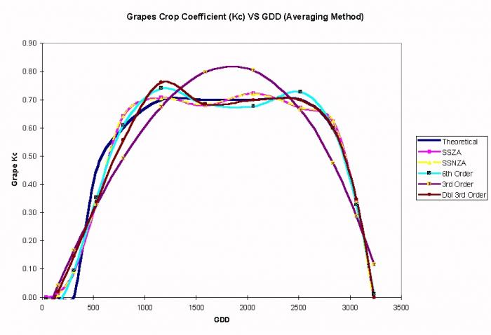
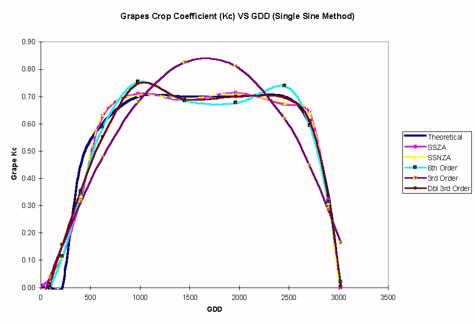
Description of Curve Fit Equations
Sine Series
* The sine series curve fits have the following form:
      o Kc= A0 + B1 * sin( T ) + B2 * sin( 2T ) + B3 * sin( 3T ) + B4 * sin( 4T )
      + B5 * sin( 5T ) + B6 * sin( 6T )

  where:
      o T is (GDD * pi/MaxGDD),
        A0 is the constant coefficient in the function parameters, and
        Bi is the ith Term coefficient.
6th Order Polynomial
* The 6th order polynomial function is:
      o Kc= A0 + B1 * GDD1 + B2 * GDD2 + B3 * GDD3 + B4 * GDD4 + B5 * GDD5 + B6 * GDD6

  where:
      o A0 is the constant coefficient in the function parameters, and
        Bi is the ith Term coefficient.
3rd Order Polynomial
* The 3rd order polynomial function is:
  o Kc= A0 + B1 * GDD1 + B2 * GDD2 + B3 * GDD3

  where:
      o A0 is the constant coefficient in the function parameters,
        and Bi is the ith Term coefficient.
Double 3rd Order Polynomial
The Double 3rd order polynomial function is a special case.
This function uses two separate 3rd order polynomials to fit the rising and falling portions of the crop coefficient curve. A switch point was chosen at approximately the mid-point of the period of the function and the first polynomial was fit the the data up to that point, while the second polynomial was fit the the remainder of the data, with the GDD accumulation reset to zero at the switch point. Both equations have the same form as the regular 3rd order equation: o Kc= A0 + B1 * GDD1 + B2 * GDD2 + B3 * GDD3
  where:
      o A0 is the constant coefficient in the function parameters, and
        Bi is the ith Term coefficient.
Another method of calculating the maximum crop coefficient is to measure the percent cover a midday and use a formula developed by Williams where kc = 0.002 + 0.017x, where x is percent shaded area. See an extension publication on this method. A photograph from above the grapevines can also be used to measure the percent cover using Adobe Photoshop software.
Remote Sensing Crop Stress
VINTAGE (Viticultural Integration of NASA Technologies for Assessment of the Grapevine Environment)
Earth Science Division, NASA Ames Research Center
Environmental Science, Technology & Policy, California State University, Monterey Bay
Numerical Terradynamic Simulation Group, University of Montana
Winegrowers worldwide have recognized for centuries that grapes harvested from different areas of the vineyard can produce wines with unique flavors. Even under constant variety and rootstock, the feel, bouquet, color, body and overall wine quality is influenced by differing physical factors within vineyard: microclimate, slope, aspect, soil type and water-holding capacity. However, mapping and monitoring of vineyard variability can pose a challenge.
Applied research was conducted to further develop the use of remote sensing and other geospatial technologies as decision support in winegrape and other high-value, irrigated agriculture. Prototype remote sensing products were developed to map vineyard leaf area, shoot "balance", block uniformity, and crop evapotranspiration. A water balance model (VSIM), during the season, or cumulative stress during specific phenological periods.
Collaborators included the Robert Mondavi Winery (Oakville, CA), VESTRA Resources, Inc. (Redding, CA) and the Bay Area Shared Information Consortium. VINTAGE was sponsored by NASA's Earth Science Program.
View and interact with remote sensing based products for a 500 acre vineyard located in the Carneros region of Napa County
See daily water balance simulation of 1000 ac Napa Valley vineyard for 2005 season
Prior research projects: GRAPES (phylloxera monitoring); CRUSH (management zones/segmented harvest)
CONTACT: Lee F. Johnson, Principal Investigator, Ljohnson@mail.arc.nasa.gov
Last update: 30-May-07